Notes - Excel

Tips

• To insert current date: Ctrl+;
• To insert current time: Ctrl+Shift+;
• To add today’s date in such a way that it updates when you recalculate or reopen your spreadsheet: =Today()

Usage

XLOOKUP

=XLOOKUP(lookup_value,lookup_array,return_array,if_not_found,match_mode,search_mode)

• lookup_value - the value to look for
• lookup_array - the range or array to search within
• return_array - the range or array to return values from
• if_not_found - value to return if no match is found
• match_mode - settings for exact, approximate, and wildcard matching
• search_mode - settings for first to last, last to first, and binary searches

Customer send asset list asking for status.

• Download Inventory All Fields file, and open it in Excel(default .CSV)
• Open customer file, copy the Inventory All Fileds page into

// H column: Label; AA column: Site
=XLOOKUP(A2,'RL Inventory All Fields'!H:H, 'RL Inventory All Fields'!AA:AA)

How to get the last non-empty value

Column J is the COGS value for each category. To get the total COGS value(last) from column J, use the following formula:

=XLOOKUP(TRUE,'Yield-Category'!J:J<>"",'Yield-Category'!J:J,,,-1)

Find an asset in another column?

Find an asset in another column, show “Yes” if found, “No” if not.

// find B1 in column A
=IF(COUNTIF(A:A,B1)>0,"Yes", "No")

// find D2 in range A:2 to A:14
=IF(COUNTIF($A$2:$A$14, D2)>0, "yes", "no") // lock the range

You can use COUNTIFS if there are multiple criteria across different ranges.

How to delete everything after space?

To change the text 12/10/2025 07:34:58 to 12/10/2025, use the following formula:

=LEFT(A1,Find(" ",A1)-1)

Q & A

How to generate barcodes in Excel?

To generate barcodes in Excel, you’ll need to use a barcode font and a formula.

• Download and install a barcode font like Code 39 or Code 128.
• Create a formula that adds starting and ending characters to your data

Suppose the Asset Tag is in cell A2, barcode is in B2.

• Type in the following formula in B2: ="*"&A2&"*" or add asterisk character before and after your text like *LPNNL4XDM5MFF*
• Apply the barcode font to cell B2.

Note: If you use barcode in Word: There is a default setting in some versions of Word that changes text surrounded by *’s into bold text. This setting must be disabled for these fonts to work, otherwise the * characters that are necessary for the barcode to scan properly will be lost and the thickness of the bars will be altered. The setting might be found in a different place in different versions but this is how I disabled it. From the Tools menu open the AutoCorrect dialog box. On the AutoFormat tab uncheck the box for “Bold and underline”

How to get the delta from previous two cells?

For the weekly report, the right most delta column is used to show the difference between the last two weeks. Each week we add a weekly column before the delta column.

To get the delta value from the last two weeks, use this formula:

// A3:ZZ3: the third row, data will be between column A and column ZZ
// COLUMN(): current column number
=INDEX(A3:ZZ3,1,COLUMN()-1)-INDEX(A3:ZZ3,1,COLUMN()-2)

How to add a link to another sheet in the document?

Insert > Link

• Text to display: Goto Sheet2
• Link to: Place in This Document
• Cell Reference: Select Sheet2

How to fill in the formula to the rest of the cells?

Suppose you have a 3-column table with header, the formula in column C2 is: =A2+B2

If there’re 10 rows with the same formula, You can select C2 to C11 and press Ctrl + D to fill the formula to the rest of the cells below C2.

The alternative is to copy C2, select the other cells and paste the formula to them.

How to insert the same data to multiple cells at the same time?

• Select all cells you want to insert the data
• Press F2 and type in the data
• Press Ctrl+Enter

How to un-hide all rows?

Using keyboard shortcuts:

• Ctrl + A: Select the entire document
• Ctrl + Shift + 9: unhide all rows on your spreadsheet

Using context menu:

• Home > Format > Hide & Unhide > Unhide rows

How to open the file in Desktop App?

When someone share a link to an Excel file, it usually opened in Browser if you click the link.

To open the file from desktop app

• Click the Editing icon on the top right corner
• Open in Desktop App

How to make a table as strap color?

Format it as a table:
Home > Format as table

If you want to use different colors for your table:
Page Layout > Theme Colors

How to add Header & Footer ?

It’s better to add the file path and name at the bottom of the Excel form so that we can find it easily in the future.

Follow these steps to add header and footer in Excel:

• Go to Insert tab, in the Text group, click Header & Footer
• Excel will display the worksheet in Page Layout view
• To add or edit a header or footer, click the left, center, or right header or footer text box at the top or the bottom of the worksheet page (under Header, or above Footer)
• Type the new header or footer text

To close the header and footer, you must switch from Page Layout view to Normal view

• On the View tab, in the Workbook Views group, click Normal.

How to view file version history?

• Open the file you want to view.
• Click File > Info > Version history.
• Select a version to open it in a separate window.
• If you want to restore a previous version you’ve opened, select Restore.

How to remove/suppress the #DIV/0! error?

Use any of the following formula to remove the #DIV/0! from Spreadsheet:

• =IFERROR(A1/A2, 0)
• =IF(A2,A1/A2,0) or =IF(A2,A1/A2,"No Input")
• =IF(ISERROR(A1/A2),0,A1/A2)

How to show data conditional?

In the daily report file, I want to show the WIP data in current date, but not in the future date.

// Show data only if tested assets(B4) and receiving assets(C4) exists
=IF((B4+C4)>0,D3-B4+C4,"")

How to paste CSV data into individual columns?

When pasting CSV data into Excel, all the data will be in one column. To separate the data into individual columns, follow these steps:

• Data > Text to Columns
• Original data type: Delimited / Fixed width
• (For Delimited)Delimiters: Tab / Semicolon / Comma / Space / Other

Caution: Excel will remember your selection and when you paste data next time, it’ll apply these settings automatically.

How to force Excel to re-calculate all the formulas?

Using keyboard shortcut Ctrl+Alt+F9 to re-calculate the workbook formulas.

• F2 – select any cell then press F2 key and hit enter to refresh formulas.
• F9 – recalculates all sheets in workbooks
• Shift+F9 – recalculates all formulas in the active sheet
• Ctrl+Alt+F9 – force calculate open worksheets in all open workbooks including cells that have not been changed
• Ctrl+Alt+Shift+F9 – recalculates all sheets in all open workbooks

How to copy and paste just visible cells only?

Keyboard shortcut:

Select the range, press ALT + ; will select only the visible cells. See here

Sort/Filter area

Sort & Filter > Filter: You can copy/paste the visible cells of the sorting area.

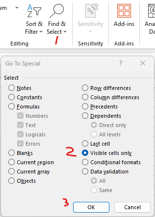
Select visible cells

• Select the entire range you need to copy.
• Home > Find & Select > Go To Special... (Or press F5 > select Special...)
• Select Visible cells only > OK
• Press CTRL + C to copy.
• Then go to target sheet and press CTRL + V to paste.

How to remove duplicated rows?

You can remove duplicate cell values or rows according to your selection.

1. Select the range of cells that has duplicate values you want to remove.
2. Click Data > Remove Duplicates, and then Under Columns, check or uncheck the columns where you want to remove the duplicates.

Note: the duplicate is for the rows you selected, it may contain one or more columns.

How to jump to the first/last worksheet directly with keyboard?

We created a spreadsheet for our 500 location labels. You can use these shortcuts to move around the worksheets.

• Ctrl + PgUp or Ctrl + PgDn: move to previous/next worksheet
• Ctrl + < or Ctrl + >: move to first/last worksheet

How to highlight duplicate values?

1. Select the cells you want to check for duplicates.
2. Click Home > Conditional Formatting > Highlight Cells Rules > Duplicate Values.
3. In the box next to values with, pick the formatting you want to apply to the duplicate values, and then click OK.

Note: This can only highlight individual duplicated cells, not duplicate rows.

Why the cell can’t show out the whole number in Text format?

Excel cell format is General by default, therefore it can display up to 11 digits in a cell. For numbers more than 11 digits it’ll show out as scientific format such as 1.23457E+11. At this time even if you apply the Text format, the whole number doesn’t show out.

You need to set the cell format as Text first, then enter the long number.

Alternatively, type a single quotation mark (’) first in the cell, and then type the long number. (such as '1234567890123)

How to fill in data into the pre-ordered associate name list?

The XLOOKUP function searches a range or an array, and then returns the item corresponding to the first match it finds. If no match exists, then XLOOKUP can return the closest (approximate) match.

1

=XLOOKUP(lookup_value, lookup_array, return_array,[if_not_found], [match_mode], [search_mode])

• The source data(User Metrics) are in column F and G
  • Employee Name in column F from F2 to F24
  • FG(Client) number in column G from G2 to G24
• The pre-ordered associate names are in column B from B2 to B31; The data will be filled into column C (C2:C31)
• Type in the following formula to C2:C31(Example C11):
  • =XLOOKUP(B11,$F$2:$F$24,$G$2:$G$24,0); This formula means search Chen, Jun(B11) in range F2:F24, if found, return data in G2:G24(10); if not found, return 0;

Excel doesn’t update formula after recent updating, how to fix it?

Excel doesn’t update formulas. Whenever I copy a formula, the value in the destination cells show the same value as the source and doesn’t re-calculate in the new cells.

Change the following settings to fix this problem:

• File > Options > Formulas > Workbook Calculation > Automatic

How to fix circular references error?

Go to tab Formulas, choose Error-checking (or Circular References on dropdown list), Excel will show out all formula errors.